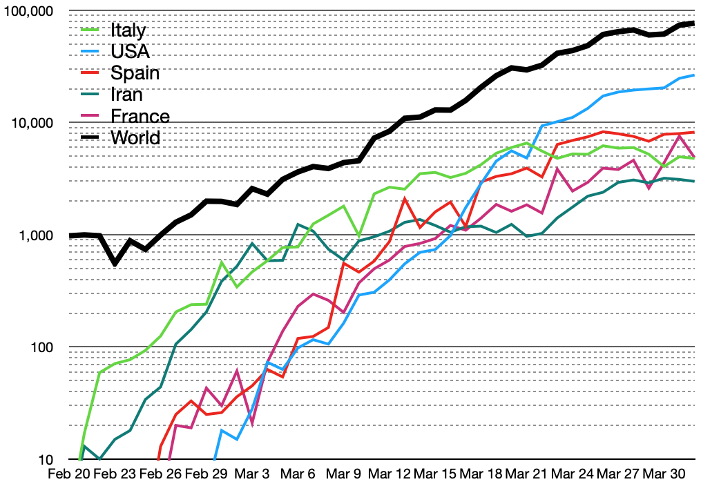
Semi-log plot of daily new cases of
COVID-19 in top five countries
and in the world --- from the
Wikipedia Covid-19 pandemic page
(World Health Organization data)
Simple Math (Arithmetic)
|
(2020 Mar blog post)
SECTIONS BELOW:
INTRO
EXPONENTIAL EQUATIONS
COMPUTATION METHOD
DATA TABLES BELOW:
! Note !
Text or web-links or images may be added
(or changed) --- if/when I re-visit this page.
|
INTRODUCTION : In January and February of 2020, the 'coronavirus' --- that broke out in China in Dec 2019 --- spread throughout the world --- with stunning reports from South Korea, Iran, Italy, and eventually the United States --- alerting the world to a world-wide 'pandemic'. There were people at the top of the U.S. government who were claiming the outbreak of the virus in the USA was a 'hoax' and 'just the flu' and 'contained' ( Donald Trump, Larry Kudlow, Kellyanne Conway, Sean Hannity, and others). (Sean Hannity seems to be Trump's 'Chief Scientist'.) In early 2020, Trump was saying there were only about 5 cases (in the state of Washington) --- and the cases were going down to zero --- and the outbreak would soon 'wash away'. These people at the highest levels of the government (including a 'stable genius' who knew more than generals and doctors and anybody else in the world) apparently
Apparently Trump --- who is known for NOT-READING books and reports --- did not read his math books either --- and, as a result, he doomed the United States to suffer many more deaths of citizens and hospital workers than would have happened if he had done some of his math homework --- instead of practicing incessant bullying. Trump does not understand the importance of 'social distancing' and 'shelter in place', which will "buy time" for 'partial' and 'full' solutions for this Covid-19 virus to 'fall into place' --- thus saving many lives. It is the intent of this web page to show how any person (including Trump) could come up with 'ball park' estimates for how an epidemic of a virulent new virus in a given region (and for a given infection rate) would grow --- and peak and decline. By 'new virus', we mean a virus for which there is no 'cure', like a vaccine, and for which the population has not built up an immunity (or partial immunity, say by some portion of the population). This scenario simplifies the development of equations for modelling the spread of the virus. And these assumptions apply to the '2019 coronavirus'. SOME DATA SOURCES Within a month after the coronavirus broke out in China, there were many Wikipedia pages on the '2019' virus --- including pages that showed bar charts of the number of new infections and deaths (a bar for each day) --- for many countries of the world --- and for states (and cities) of the United States. Examples:
U.S. GOV. RESPONSES - Jan,Feb 2020 In the sections below, this page presents some basic math (arithmetic = addition and multiplication) that provides any person with rough estimates of how an epidemic proceeds --- for any given (average) infection rate, or death rate. But before we get to the math, you might want to try a few web searches to see how we (in the United States) got to be the most-highly-infective-country-in-the-world --- due to late 'federal' responses and horrible 'federal' decisions. ( MAGA = "Make America Germophobic Again") (The United States cases are plotted using the blue line in the graph below. USA ... number one, number one.) |
Semi-log plot of daily new cases of
COVID-19 in top five countries
and in the world --- from the
Wikipedia Covid-19 pandemic page
(World Health Organization data)
|
To discover the truth about how the Trump administration fiddled while the virus burned through the population, you can try WEB SEARCHES on keywords such as
Alternative searches: In doing web-searches like these in 2020, I found that there are so many right-wing and conspiracy-theory-promoting sites trying to "re-write history", that searches like these may yield more bullshit-sites than truth-sites. So, to find some "just the facts" sites, you can try some of the searches above --- and then change some of the keywords --- for example, to reference specific wording in quoted remarks. For example, since Larry Kudlow was repeatedly saying "nobody could have predicted or expected this" on 23 March 2020 on CNBC --- and CNBC was repeatedly playing the audio of this quote going into commercial breaks in March 2020 (thanks a lot for spreading Trump's lies, CNBC) --- you could try WEB SEARCHES on keywords like:
The web searches and comments above show that Trump, Pence, et. al. wasted at least 2 months claiming this virus was 'just the flu' --- while the virus was spreading exponentially, building up its base --- when they should have been doing things like
But ... after more than 2 months of delays, Trump still devoted essentially all of his efforts into denials and trying to re-write history. Not just delays --- also dismantling What is perhaps even worse than the delays is the fact that soon after Trump became President in 2017, his 'aides' --- Mick Mulvaney and Stephen Miller --- went through the various U.S. Goverment departments, agencies, and bureaus --- to un-do anything that had been started by President Obama. In the process, they (or, reportedly, John Bolton) did away with a 'pandemic response group' that had been started in response to outbreaks of viruses such as SARS-CoV-1, Swine Flu, MERS, Ebola, and Zika. So Trump wiped out the team and individuals that could have provided critical planning and execution that would have helped "flatten the curve" of daily new infections --- thus gaining valuable time to put into place critical medical supplies and to develop and test new therapies and drugs and vaccines --- and thus saving thousands of lives. Trump can't change ... Trump promotes Trump
(It's his highest priority. Since Trump continued saying "no one knew the virus ..." and "nobody knew the virus ..." into March and April 2020, you could try searches like: With these searches, you may find many of his 'no one knew' statements over the years (on subjects other than this virus). Trump is fond of saying 'no one knew' --- with the implication being 'only he knew'. At least 50% of the people of the U.S. know that you do not know much of anything about the many things you claim to know, Donald. Whenever Trump says "no one knew", that means "Donald Trump did not know --- but plenty of other people knew". Trump is proving to be useless to everyone but himself in this pandemic. |

|
MATH FOR EXPONENTIAL GROWTH The math for exponential growth is based on a simple equation that says that the 'rate of change' of the 'population count' of an 'item' is changing in proportion to the current number of that item (examples: humans in an epidemic, atoms in a chain reaction). In compact math form: dx/dt = R * x where 'x' is a number representing the current count of the population and 'R' is a 'proportionality constant' that affects the rate of growth (or rate of decline if 'R' is negative). The symbol 'dt' represents a time step --- and 'dx' represents the change in the population count over one instance of that time step. The symbol 'dx/dt' represents a ratio --- the change of the population count per step in time. It can be thought of as the 'velocity or speed' of change of the population count. Let us consider the case of R = 2.0. It may help to think of dt as one unit of time. Then, for dt = 1, the equation above becomes dx = R * x. This equation says that 'dx' (the change in the population) is equal to 'R * x' --- over one time step. For R = 2.0, 'the population change' (dx) in one time step is double the current population count (x). We will be letting 'x' be the count of a number of 'infected' people in a population in a region, rather than a count of the entire population. (The 'total infected population count', x, will actually be tripling over each time step for R=2.0, as we will see below. For R=2.0, we will be modelling the fact that the 'new cases' --- that is, the 'CHANGE in the population of infecteds' --- over the next time step is given by doubling the current 'total infected population'. So, with R=2.0, we are modelling the case of, on average, each infected person causing the creation of two NEW infected people, over the next time step.) For the case of a virus epidemic, a suitable time step would be in 'weeks' rather than 'days' or 'hours' or 'minutes' --- because the data for determining the rate constant (R) is typically fluctuating quite a bit from day to day. Also, by using 'weeks' rather than 'days', we can 'minify' the number of computations as well as the size of the resulting data tables. In fact, the factor 'R' is typically not constant, but can vary over time as situations such as 'social distancing' and 'migration of infectives over boundaries' affect that rate. However, we can get quite useful 'ballpark' predictions based on an 'average' value of the factor 'R'. METHOD OF NUMERICAL COMPUTATION The 'rate equation' shown above is one of the simplest forms of what is known as a 'differential equation'. We think of the unknown 'x' as a 'function of time' --- typically denoted 'x(t)'. And we want to generate values for 'x' at various times 't'. To use that 'rate equation' to make numerical predictions, we actually use it in a different form: dx = R * x(t) * dt This equation says that the 'change in x' (near a given time 't') is the product of R and x(t) and dt. For predictions of growth/change in epidemics, it is typical to use dt = 1 --- such as one week (or one day or one month). So, for computational purposes, we use the simple equation: dx = R * x(t) where 'R' must be based on the same time-units as 'dt'. The equation above gives a number 'dx' representing a change in 'x' near a time 't'. However, that does not give us 'x' at a next time step. For that, we need an additional very simple equation: x(t+dt) = x(t) + dx This equation simply says that the value of 'x' at a 'next time step' is given by the value of 'x' at the 'previous time step' PLUS the change in 'x' that we got from the rate equation: dx = R * x(t) STARTING THE COMPUTATION OK. So now we have the two simple equations that we will use to generate x(t) at various times --- t, t + dt, t + 2*dt, t + 3*dt, ... The two simple equations are
dx = R * x(t)
But now we need a bit of data to start the computation. This bit of data is called an 'initial value' or 'initial condition'. In general, we can think of wanting to generate a table of values of 'x' at times t0, t1, t2, t3, ... And, in our 'constant-time-step' case:
t1 = t0 + dt, where dt = 1 (week, say). Then, to start off our computation, we need a value of 'x' at initial time 't0' --- denoted x(t0). Then we simply start computing, using the pair of equations above, over and over:
dx = R * x(t0)
dx = R * x(t1)
dx = R * x(t2)
and so on. For simplicity, we will let t0 = 0. Then as we successively add dt = 1 to t0, we get t1 = 1, t2 = 2, t3 = 3, ... Then, with this 'one unit time step', the pairs of equations above become:
dx = R * x(0)
dx = R * x(1)
dx = R * x(2)
and so on. |
|
A PREDICTION BASED ON R=2.0 The following table is one that I generated based on the fact that, in mid-March 2020, there were said to be about 5,000 reported cases of infections, in the United States, from the 2019-coronavirus (COVID-19). From some of the limited data at that time, it looked like the number of infections were (at the very least) doubling every week. So I decided to see what the initial growth rate of infections would look like for R = 2.0 in our 'computational equations' above. In this case, our 'x(t)' will denote the number of total reported COVID-19 infections at time 't' --- in the United States. Note that at week-zero, we start with the value x(0) = 5K. We double that to get dx = R * x(0) = 2.0 * 5K = 10K. Then, to get x(1), we use x(1) = x(0) + dx = 5K + 10K. And we continue that pattern. To make these computations look simpler, we could combine our 2 'computational equations' into one:
x(i+1) = x(i) + dx = x(i) + R * x(i)
Note that this computation can be simplified from one multiplication and one addtion to a single multiplication:
x(i+1) = (1 + R) * x(i)
So each entry in the last column of the table is simply 3.0 times the previous entry in that column. |
   ---------------------------------------------------------------
   Virus Infection Simulation
   (Rate R = 2.0 per week ; i.e. doubling 'x' gives 'dx')

           (dx=R*x)         ( x(i+1)=x(i)+R*x(i) )
  End of    Added            Cumulative
   Week   Infections       Total Infections
  Number  (2xPrev.week)  (Prev.week + This week's increase)
  ------  ----------   -----------------------------------
    0        0            5K                      mid-March
    1       10K           5K +     10K = 15K
    2       30K          15K +     30K = 45K
    3       90K          45K +     90K = 135K
    4      270K         135K +    270K = 405K     mid-April
    5      810K         405K +    810K = 1215K
    6     2430K        1215K +   2430K = 3645K
    7     7290K        3645K +   7290K = 10935K
    8     21870K      10935K +  21870K = 32805K   mid-May
    9     65610K      32805K +  65610K = 98415K
   10    196830K      98415K + 196830K = 295245K
                                  nearly 330000K = U.S. population
The lower graph is the NEW cases,
i.e. new infections for each week.
The upper graph is the CUMULATIVE cases,
i.e. the cumulative infections.
|
Note that at 8 weeks (two months after mid-March = mid-May 2020), this table predicts that there may be on the order of 33 million reported infections in the United States --- out of a population of about 330 million. So, at 8 weeks (mid-May 2020), about 33/330 or about 10 percent of the population of the U.S. may have experienced infection. Note that this means that about 90% of the population may still be susceptible to infection. And, stepping back a month, this table predicts that there may be on the order of 405 thousand reported infections in the United States in mid-April. So, at 4 weeks (mid-April 2020), only 405,000/330,000,000 = 0.0012 --- or ONLY about one-tenth of one percent of the population of the U.S. may have experienced infection --- EVEN THOUGH 405,000 infections sounds like a LOT OF INFECTIONS. This means that more than 99% of the population may still be susceptible to infection. In sections below, a modification of our 'computational equations' will be presented to take into account that this exponential growth cannot go on forever. There are a limited amount of 'susceptibles' in the population as more and more of the population becomes infected. But, before we take on that 'enhancement' of our predictive equations, let us consider the 'initial' form of the 'curve of deaths'. DEATH PREDICTIONS Some of the initial data from the United States indicated that the number of deaths per number of infected was about one percent. This 'death-percentage' may be rather optimistic. In some areas of the U.S. and in some countries, it looks like the death-percentage may be more like 3 or 6 percent. (In some nursing homes, the 'death-percentage' is on the order of 50 percent.) Using that fact (rough estimate), we can generate the following table to provide a 'curve of deaths'. |
   -----------------------------------------------------------
   Deaths resulting from the virus with Infection Rate
   R = 2.0 per week (i.e. doubling of 'x' gives 'dx')

  End of  ( x(i+1)=(1+R)*x(i) )
   Week     Cumulative Total    Cumulative Total Deaths
  Number      Infections        (1% of Cum. Infections)
  ------   -----------------    -----------------------
    0         5K                 50         mid-March
    1         15K                150
    2         45K                450
    3         135K               1350
    4         405K               4050       mid-April
    5         1215K              12,150
    6         3645K              36,450
    7         10935K             109,350
    8         32805K             328,050    mid-May
    9         98415K             984,150
   10         295245K            2,952,450
The lower graph (near the x-axis) is the
CUMULATIVE DEATHS, assuming that about
1 percent (1/100th) of infections result in death.
The upper graph is the CUMULATIVE CASES,
i.e. the cumulative infections.
The cumulative deaths curve looks very low
relative to the cumulative-infections curve
--- but deaths will trend toward 2 million total,
not an insignificant figure for those 2 million
people --- and their relatives and friends.
The cumulative infections curve gives an idea
of how badly hospitals could be overwhelmed.
NOTE:
The wearing of masks and social distancing would
result in a much lower infection rate --- thus
'flattening' the cumulative infections curve ---
as it has been flattened in countries like South Korea
and Japan, countries that learned some lessons
from past SARS outbreaks.
|
This table suggests that the number of deaths in the United States from COVID-19 would be on the order of 4,000 by mid-April 2020. And, by mid-May 2020, the number of deaths could be on the order of 330,000. A PREDICTION BASED ON R=4.0 Soon after I generated the table above (for doubling of infections every week), I noticed --- in the data (bar graphs) for cumulative infections in the United States (at the U.S. coronavirus page at Wikipedia) --- that the infections were doubling about every 3 to 4 days --- not every 7 days. So I decided to generate a table for that situation --- of a doubling in infections every 3.5 days. That situation implies that we should, perhaps, use R = 4.0 in the 'computational equations' above. In case you ask 'why 4.0?', here is why: Say you have 100 infected people at the start of the week. Then 3.5 days later, you will have 2 * 100 = 200 infected people. And then 3.5 days later, you will have 2 * 200 = 400 infected people. So you started at the beginning of the week with 100 infected people --- and you end up at the end of the week with 400 infected people. Hence, every week, the number of infected goes up a factor of 4.0. (Actually, we should determine R by noting that dx/dt = R * x can be rearranged to R = dx / x when dt = 1. So we should evaluate R as the 'change in x over x'. In this case, it would be
R = dx / x = (x(i+1) - x(i)) / x(i) =
So R = 3.0 at that one week. But let us 'go big' and use R = 4.0.) In generating this table, we will reduce the number of operations necessary by noting what we observed above: Namely, the two 'computational equations'
dx = R * x(t)
which involve a multiplication and an addition, can be simplified to a single equation
x(i+1) = x(i) + R * x(i) For R = 4.0, we get the equation x(i+1) = 5.0 * x(i) which involves a single multiplication. And that gives us the following table. |
   -------------------------------------------------------------------
   Virus Infection Simulation
   (Rate R = 4.0 per week ; i.e. quadrupling 'x' gives 'dx')

              ( x(i+1)=(1+R)*x(i) )
  End of          Cumulative                  Cumulative
   Week        Total Infections              Total Deaths
  Number    (5.0 times the Prev.week)     (1% of Cum. Infections)
  ------   ----------------------------   -----------------------
    0                 5K                   50         mid-March
    1                25K                   250
    2               125K                   1,250
    3               625K                   6,250
    4             3,125K                   31,250     mid-April
    5            15,625K                   156,250
    6            78,125K                   781,250
    7           390,625K  <--- past the
    8         1,953,125K      population of U.S.
    9         9,765,625K
   10        48,828,125K
The lower graph (near the x-axis) is the
CUMULATIVE DEATHS, assuming that about
1 percent (1/100th) of infections result in death.
The upper graph is the CUMULATIVE CASES,
i.e. the cumulative infections.
NOTE:
This R=4.0 infection rate is quite high, perhaps
even higher than the initial rate in New York City.
With wearing of masks and social distancing,
a cumulative curve this steep can be avoided.
|
Note that at 4 weeks (one month after mid-March = mid-April 2020), this table predicts that there may be on the order of 3 million reported infections in the United States --- out of a population of about 330 million. So, at 4 weeks (mid-April 2020), about 3/330 or ONLY about 1 percent of the population of the U.S. may have experienced infection --- EVEN THOUGH 3 million infections sounds like a HUGE NUMBER OF INFECTIONS. Note that this means that about 99% of the population may still be susceptible to infection. And, advancing down the table, it appears that at week 7 (about the 1st week of May 2020) the entire United States more than 300 million people) will have been infected. This implies there is an EXPLOSION of infections in weeks 5, 6, and 7 --- the end of April and early May. HOWEVER, there are at least a couple of reasons why the infection rate will slow down into May.
A PREDICTION BASED ON R=5.0 Soon after I generated the tables above (for doubling AND quadrupling of infections every week), I noticed --- in the data (bar graphs) for cumulative infections in the United States (at the U.S. coronavirus page at Wikipedia) --- that, in mid-March, there were about 4 days when the infections were increasing between about 23% and 30% each day. I decided to check how that translated into a weekly growth rate factor, R. I decided to use an estimate of 1.26 for the daily increase in infections from the previous day. Then over seven days, one week, the growth rate factor at the end of each day is seen to be given by:
where the '^' symbol indicates exponentiation. (As Trump would say: "A very big word.") So this implies that a 26% daily jump in infections over a 7 day period results in a factor of 5.0 increase in the 'infected total' over each week (assuming that strategies like 'social distancing' do not reduce that rate --- and assuming that 'migration of infectives into the region' do not increase the rate). So the question now is "what value of R should we use based on this data?" We noted above that, in our model of exponential growth, x(i+1) = (1 + R) * x(i) We can rearrange this to solve for R, giving R = ( x(i+1) / x(i) ) - 1 So, say we started at the end of week 'i' with x(i) = 100 cases. Then our observation above is that at the end of week 'i+1', we would have about x(i+1) = 5.04 * 100 = 504 cases. Plugging into the formula for R, we get R = (504 / 100 ) - 1 = 5.04 - 1 = 4.04 This suggests that we could use R = 4.0 for a 'simulation run' based on the 26% daily increase in cases. But we did a run, above, for R = 4.0. Let us see what happens when R = 5.0. Like we did in generating some tables above, we use the following equation to generate a table of values for x(i) --- the number of infected people at the end of week 'i'. x(i+1) = x(i) + R * x(i) = (1 + R) * x(i) For R = 5.0, we get the equation x(i+1) = 6.0 * x(i) which involves a single multiplication. And that gives us the following table. |
   ------------------------------------------------------------------
   Virus Infection Simulation
   (Rate R = 5.0 per week ; i.e. quintupling 'x' gives 'dx')

              ( x(i+1)=(1+R)*x(i) )
  End of           Cumulative                  Cumulative
   Week         Total Infections              Total Deaths
  Number      (6.0 times the Prev.week)     (1% of Cum. Infections)
  ------   ----------------------------   -----------------------
    0                 5K                   50         mid-March
    1                30K                   300
    2               180K                   1,800
    3             1,080K                   10,800
    4             6,480K                   64,800     mid-April
    5            38,880K                   388,800
    6           233,280K                   2,332,800
    7         1,399,680K  <--- far
                          past population
                          of U.S. which is
                          about 330,000K
The lower graph (near the x-axis) is the
CUMULATIVE DEATHS, assuming that about
1 percent (1/100th) of infections result in death.
The upper graph is the CUMULATIVE CASES,
i.e. the cumulative infections.
NOTE:
This R=5.0 infection rate is quite high,
perhaps higher than will be experienced
anywhere in the world with Covid-19.
But a future mutation of this virus --- or
an even more virulent virus like MERS ---
could have an infection rate this high.
|
Note that, like with R = 4.0, for R = 5.0, we see that we reach infection of the population of the entire United States between weeks 6 and 7 --- about a month-and-a-half past mid-March --- in early May. See the discussion after the R = 4.0 table for reasons why we need to 'enhance' the equation we are using to simulate the growth in the number of 'infecteds' --- in order to generate a curve with an 'apex' in the weekly number of 'new infecteds' (dx) --- and a 'levelling off' of the curve for the cumulative number of infecteds, x(t).
Perspective on the growth rates, R These rate values (R = 2.0 to 5.0, weekly) are extremely high growth rates --- as can be seen by comparing to the human population growth rate on Earth. The World Population Growth (MORE than Exponential) web page on this site points out that the population of humans on the Earth is growing at a rate of about 2 to 3 percent per year. We could get a rough 'per week' growth rate from this by dividing 0.03 by 52 (weeks), giving 0.000577. Due to the compounding effect, we really should use a somewhat lower WEEKLY growth rate of 0.000568 --- but that difference does not matter much in this discussion. Note that a 0.00057 weekly growth rate is immensely smaller than the weekly growth rates of 2.0 to 5.0 that are typical to this Covid-19 infection. Those Covid-19 rate factors R = 2.0 to 5.0 correspond to one infected person passing the infection on to about 2 to 5 people PER WEEK, on average, for the population in a region. These are much higher rates than about 3 babies PER YEAR being born per 100 people on Earth --- or, expressed on a per-person basis, each person generating about 0.03 babies PER YEAR --- or about 0.000568 babies PER WEEK. And, indeed, the kind of exponential growth of the human population over DECADES is accomplished in WEEKS by 'infecteds' in the Covid-19 pandemic. The bottom line here is that the growth rate of 'infecteds' in the Covid-19 pandemic is MUCH MUCH HIGHER (by a factor of about 10,000) than the birth rate of mammals, like humans.
A May 2020 Update on the infection rate, R In the mid-April to mid-May time frame, the use of social distancing and wearing of masks was taking hold --- partly due to the daily 'hospital chats' of Governor Cuomo of the State of New York. Also, the CDC, who initially (in February) told people not to wear masks, FINALLY told people to wear masks. (They were probably trying to avoid a rush on masks that would make it hard for hospitals to get proper masks. But that advice was counter to what Asian countries learned from previous outbreaks of SARS and other viruses.) The wearing of masks (and 'social distancing' and 'shelter in place') will have the effect of reducing the infection rate of Covid-19 significantly. It may be the case that values of R that would take into account these actions would be in the range of about 0.1 to 1.0. The simulations above could be re-done when it is clearer what a suitable value of R would be when masks and social distancing are practiced.
TO BE CONTINUED At this point, I pause to publish this page as-is. In coming days, I plan to provide
Since this page is getting rather long, I will present these subject-items on a separate web page:
Math for Epidemic GROWTH-AND-DECLINE |
|
For further information : In case I do not return to update this page, here are a few keyword WEB SEARCHES that you can use to provide updates. |

|
Bottom of this page on
To return to a previously visited web page location, click on
the Back button of your web browser, a sufficient number of times.
OR, use the History-list option of your web browser.
< Go to Top of Page, above. >Or you can scroll up, to the top of this page. Page history:
Page was created 2020 Mar 31.
|